The Gray Scott Model of Reaction Diffusion is an interesting instance of emergence. By simulating a small chemical system that involves only a few components and reactions, complex and mesmerizing patterns appear.

You can interact with the simulation above by clicking on it to drop some green and you can reset it by pressing the previous (⏮️) button.

Although the local rules and the underlying math are quite simple, there is some heavy computations involved. For each time step in the simulation, we must apply these rules to compute the concentrations of every involved component at every possible location. Running such a simulation on a CPU would be extremely slow. GPUs, however, are specifically built to handle large volumes of a single small computation in parallel.

This post is an introduction to writing such simulations using GLSL ES, with a basic implementation of the Gray Scott model that runs in the browser on Shadertoy that is less than 100 lines of code.

1. Prerequisites
   1. Computing simulations
   2. Gray Scott model
      1. Chemical reactions
      2. Diffusion
      3. Catalytic reactions
      4. Auto-catalytic reactions
      5. The Gray-Scott model itself
   3. Shaders
      1. What is a shader ?
      2. The basics of writing shaders
2. Implementing the simulation
   1. Update rules
      1. Reactions
         1. Auto-catalytic reactions
         2. Gray-Scott reactions
      2. Diffusion
   2. Visual representation of the system
   3. Texture buffer
   4. Simulation shader
      1. Initialization
      2. Update rules implementation
      3. Final shader
3. Playing with the simulation
   1. Interesting emergent behaviors
   2. Hacking on the code
   3. Continuous cellular automata
4. Conclusion

Prerequisites

In this section, I’ll try to quickly introduce some important concepts in a short and beginner friendly way.

Computing simulations

Simulating any kind of physical system involves computing what happens at any possible location, for any possible moment in time.

However, the world we live our daily lives in is continuous in regards to space and time : the real world is not made in a voxel grid of even the smallest size. Likewise, even the shortest durations can still be split into smaller durations. Worded differently, any volume larger than 0 contains an infinite amount of points in space, and any duration larger than 0 contains an infinite amount of points in time.

Computers cannot simulate a continuous world because it would require infinite computations to handle even the tiniest fractions of space and time. To overcome this, we will discretize both space and time.

Discretization is the action of subdividing space into a fixed grid, and time into fixed elementary durations (time steps). For each cell of this grid, we will repeatedly run a computation to determine how its content changes over one time step. This results in an approximation of a continuous world. The smaller our grid and time steps, the more accurate our simulation.

Since we will be using shaders, which is a technology from computer graphics, it makes sense to use pixels as grid cells, and frames (as in frames per second) as elementary time steps. (The simulation we will build will run in a 2D space for easier visualization and manageable computations).

In the following, I’ll use \(dT\) to represent the duration of an elementary time step. \(dX\) and \(dY\) will be the size of a single grid cell. Elementary lengths and durations in discrete spaces are usually written with the \(\Delta\) prefix, but using \(d\) instead will make it consistent with the code.

Gray Scott model

The Gray Scott model describes a specific family of reaction-diffusion systems. More specifically, they involve an auto-catalytic reaction. Let’s first define and mathematically describe these terms. This will allow us to derive general update rules for reaction-diffusion models. Then I will describe what makes the Gray-Scott model interesting as a specific instance of reaction-diffusion.

Chemical reactions

A chemical reaction is the process in which one or more chemical species (reactants) are consumed to produce one or more other chemical species (products).

Chemical reactions are usually described with an equation that summarizes their outcome, such as the following :

\(A + 2B \rightarrow 4C\)

In this example, the reaction that is described produces 4 molecules of the \(C\) chemical species by consuming 1 molecule of \(A\) and 2 molecules of \(B\).

The speed at which a chemical reaction occurs is defined as the quantity of molecules that get transformed in a given amount of time. Every reactant (molecule that is listed on the left side of the equation) need to meet at the same time and spot for the reaction to happen. Since the probability of finding a molecule at any given spot is proportional to its concentration, the speed of the reaction is proportional to the concentration of every reactant.

The speed of the example reaction above is then :

\(speed = k*[A]*[B]*[B]\)

where \([X]\) is the concentration of molecule \(X\), and \(k\) is a positive constant we’ll call the “speed constant of the reaction”. Since 2 molecules of \(B\) are required at the input of the reaction, it needs to appear twice in the formula for the reaction speed.

Diffusion

Diffusion is the process through which certain quantities, such as chemical species concentrations, tend to spread out and homogenize. It can be easily observed by putting a drop of ink into a glass of water.

One way to think about it in the context of the simulation is that each cell of the 2D grid is slowly and constantly leaking a fixed proportion of its content to its neighbors. At the same time, it’s receiving content leaked from its neighbouring cells. We will write \(\tau_X\) as this fixed proportion for chemical species \(X\) that leaks over a base unit of time, and we will call it the diffusion rate.

Let’s consider two simple cases to make sure this is a reasonable way to model diffusion :

• If the quantity is homogeneous over the grid (the same in every cell), the outgoing amount will be the same as the incoming one, resulting in the quantity staying homogeneous.
• On the other hand, if a cell \(C_1\) contains more than a neighbor cell \(C_2\), then \(C_1\) will leak a larger amount to its neighbors than \(C_2\). This will cause the quantity inside \(C_1\) to decrease, while the quantity inside \(C_2\) will increase. In the end, quantities inside \(C_1\) and \(C_2\) are closer together than they were at the start, which is consistent for a process that homogenizes quantities.

Catalytic reactions

Some chemical reactions require a specific chemical species, which does not seem to get consumed by the reaction, to be present for the reaction to happen. Let’s consider a very simple reaction where a species \(A\) transforms to species \(B\) :

\(A \rightarrow B\)

If this reaction only happens when a third species \(C\) is present, we say that \(C\) is a catalyst for this reaction, and the reaction is said to be catalytic. While the outcome of the reaction does not affect the concentration in species \(C\), we can still make it appear in the reaction’s equation to account for its role. We do this by making it appear on both sides of the arrow :

\(A + C \rightarrow B + C\)

This changes the formula for speed of the reaction to :

\(speed = k * [A] * [C]\)

If \(C\) is absent, then \([C]=0\), making the speed 0 as well. This is consistent with \(C\) being a catalyst for the reaction. This also implies that while the concentration in \(C\) does not change during the reaction, the speed of the reaction is proportional to the concentration of species \(C\).

Auto-catalytic reactions

Among the family of catalytic reactions, there are special cases where the catalyst is also a product of the reaction : the reaction requires the catalyst to be present in order to happen and produces more of the catalyst in turn. Such reactions are called auto-catalytic reactions. The equation still makes the catalyst appear on both sides, but in this case, the number in front of it will be larger on the right side, indicating an increase in concentration for the catalyst. For instance :

\(2A + C \rightarrow 2C\)

Autocatalytic reactions are of special interest because of their role in biology and their supposed role in the origin of life.

The Gray-Scott model itself

I previously referred to the Gray-Scott model as a “Reaction-Diffusion model for a specific auto-catalytic reaction”. This means that in this model, both diffusion and an auto-catalytic reaction will happen simultaneously. The main reaction involves two chemical species \(A\) and \(B\) which react according to the following equation :

\(A + 2B \rightarrow 3B\) with speed constant \(S\)

We also consider two hypothetical reactions :

• \(\emptyset \rightarrow A\) which constantly adds species \(A\) at rate \(F\)
• \(B \rightarrow \emptyset\) which removes \(B\) with speed constant \(K\)

We call \(F\) the feed rate and \(K\) is the kill rate. If we look at the main reaction as \(A\) being used as food by \(B\), \(F\) is indeed the rate at which we add food to the system, and \(K\) is the rate at which we remove – or kill – \(B\).

Let’s also add a process that removes a fixed fraction of \(A\) and \(B\) from every cell at each time step. We will use the value of the feed rate as a speed constant for this process.

Diffusion, occurring concurrently with these reactions, is crucial for complex patterns to emerge. It will allow \(B\) to propagate through space, starting the autocatalytic reaction in new grid cells which did not previously contain any of the chemical \(B\). Diffusion will also let \(A\) flow from regions where it is more abundant to regions where it is rarer (because it was consumed by \(B\)).

By tuning the relative values of \(S\), \(F\), \(K\), \(\tau_A\) and \(\tau_B\), different kind of complex patterns can emerge.

Shaders

Shaders are a specific kind of computer programs that are designed to run on a Graphical Processing Unit (GPU). They are generally written in a dedicated programming language and are mostly used to control how a 3D world is rendered to a 2D screen.

Since good resources on how to start writing shaders already exist, this introduction will focus on the most relevant parts for implementing a Gray-Scott simulation.

What is a shader ?

Most shaders come in one of two flavors : vertex shaders and fragment shaders. Rendering a 3D world to a 2D screen roughly involves two steps :

• Convert coordinates from the 3D space to a position on screen. This involves performing a projection depending on the position of the camera. Vertex shaders perform this step
• Determine the color of each fragment (pixel) on the screen. This involves running computations on the output of the previous step for every pixel of the screen, which is what fragment shaders are made for.

Running a computation for every pixel should remind you of how we derived update rules that should be applied to every cell of a grid. By implementing such a simulation as a fragment shader, we will take advantage of the main strength of GPUs : parallelization.

While there surely exists a better way to run simulations on the GPU, the amount of resources dedicated to learning computer graphics made it a lot easier (to me) to start writing and running code on the GPU. There are even web-based editors (such as Shadertoy which I used for this) that let you compile and run your shaders in the browser without having to install anything. As a bonus, this is agnostic of the GPU brand (by contrast with Cuda which is Nvidia specific, or ROCm for AMD).

The basics of writing shaders

As I am not a shader expert, I will focus on how to get one running on Shadertoy. My understanding is that there is a lot of boilerplate that Shadertoy handles and that it is the most straightforward way to begin writing shaders.

GLSL, like most programming languages, uses variables, functions, conditionals and loops. Assuming you already used a few different programming languages, you will probably be comfortable with reading and tinkering with shader code. However, there are some specificities of OpenGL Shading Language (GLSL) that may surprise you.

The most important thing to understand is that we are going to write a function that will be run on the GPU for every pixel of every frame. This function will take the coordinates of a pixel as an input, and will output the color that should be used for this pixel. For our simulation, this means that this function will be in charge of simulating one grid cell for one time step. It will then be repeatedly executed, resulting in the full animated simulation.

Using Shadertoy, this function will look like the following :

void mainImage( out vec4 fragColor, in vec2 fragCoord )
{
    // Normalized pixel coordinates (from 0 to 1)
    vec2 uv = fragCoord/iResolution.xy;

    // Time and space varying pixel color
    vec3 col = 0.5 + 0.5*cos(iTime+uv.xyx+vec3(0,2,4));

    // Output to screen
    fragColor = vec4(col,1.0);
}

There are a few things to notice already. First, this function does not return anything. Instead, the pixel’s color is output by setting the value of fragColor, which is defined as an out parameter of the function.

You may also notice the use of variables which were not previously defined, such as iResolution or iTime. These variables are called uniforms, and their values are provided from the outside of the shader. This is part of the boilerplate that Shadertoy handles for us.

Shaders usually make heavy use of vectors, which can have 2, 3 or 4 dimensions. The sample code above features the vec* types for all three sizes of vectors. GLSL comes with a convenient syntax for picking and rearranging vector components. If we have x = vec4(0.0, 0.2, 0.4, 0.6), then x.xyy will be equal to vec3(0.0, 0.2, 0.2). You can reference each vector coordinate by x, y, z and w respectively. Since vectors are also used to represent colors, the symbols r, g, b and a can also be used.

Implementing the simulation

Update rules

This is the most math-heavy section of the article, in which we derive the update rules for the simulation.

Reactions

In the general case, when simulating the reaction \(A + 2B \rightarrow C\) for a single time step, the concentrations of \(A\), \(B\) and \(C\) need to be updated in the following way for every \((x,y)\) cell in the simulation :

\([A](t+dT,x,y) = [A](t,x,y) - speed(t,x,y)*dT\) \([B](t+dT,x,y) = [B](t,x,y) - 2*speed(t,x,y)*dT\) \([C](t+dT,x,y) = [C](t,x,y) + 4*speed(t,x,y)*dT\)

Replacing \(speed(t,x,y)\) with its expression from above yields :

\([A](t+dT,x,y) = [A](t,x,y) - k*[A](t,x,y)*[B](t,x,y)^2*dT\) \([B](t+dT,x,y) = [B](t,x,y) - 2*k*[A](t,x,y)*[B](t,x,y)^2*dT\) \([C](t+dT,x,y) = [C](t,x,y) + 4*k*[A](t,x,y)*[B](t,x,y)^2*dT\)

where \( dT \) is the duration of a time step. Notice that the numbers in front of \(speed(t)\) come from the quantities in the equation that summarizes the reaction.

Looking closely at this update rule, you may notice that chemical reactions happen independently in each cell. This can be evidenced by the fact that the formula for updating cell \((x,y)\) only involves coordinates \((x,y)\) and ignores concentrations in neighboring cells (such as \((x+dX,y)\)).

Auto-catalytic reactions

Consider the following auto-catalytic reaction :

\(2A + C \rightarrow 2C\)

The update rule for this reaction is then

\([A](t+dT,x,y) = [A](t,x,y) - 2*k*[A](t,x,y)^2*[C](t,x,y)*dT\) \([C](t+dT,x,y) = [C](t,x,y) + (2-1)*k*[A](t,x,y)^2*[C](t,x,y)*dT\)

Gray-Scott reactions

By combining the update rules for all processes (which consists in successively applying them) previously described, we get the following update rules for the “reactions” part of our Gray-Scott model :

\([A](t+dT) = [A](t) + (F - S * [A](t) * [B](t)^2 - F * [A](t)) * dT\) \([B](t+dT) = [B](t) + (S * [A](t) * [B](t)^2 - K * [B](t) - F * [B](t)) * dT\)

which can be rearranged as :

\([A](t+dT) = [A](t) + (F * (1-[A](t)) - S * [A](t) * [B](t)^2) * dT\) \([B](t+dT) = [B](t) + (S * [A](t) * [B](t)^2 - (K+F) * [B](t)) * dT\)

Diffusion

We can write the following equations for a “two-cell” system :

• The amount leaked out of a cell \(C_y\) over duration \(dT\) is \(out_X(t,C_y) = \tau * [X](t,C_y) * dT\).
• Anything that leaks out of a cell \(C_y\) gets inside the other cell \(C_z\) : \(in_X(t,C_z) = out_X(t,C_y)\)
• The variation of quantity in a cell \(C_y\) is the difference between the quantity that leaked in and the quantity that leaked out : \([X](t+dT,C_y) - [X](t,C_y) = in_X(t,C_y) - out_X(t,C_y)\) for \(y=1\) and \(y=2\)

By rearranging these equations, we get the following update rule for diffusion :

\([X](t+dT,C_y) = [X](t,C_y) + \tau_X * [X](t,C_z) * dT - \tau_X * [X](t,C_y)) * dT\) \([X](t+dT,C_y) = (1-\tau_X * dT) * [X](t,C_y) + \tau_X * dT * [X](t,C_z)\)

with \((y,z) = (1,2)\) or \((y,z) = (2,1)\).

This update rule can be generalized from a two-cell system to the 2D grid by replacing \([X](t,C_z)\) by a (possibly weighted) average of the concentrations in the neighbor cells.

Visual representation of the system

Before starting to write code, let’s pick a way to display the state of the simulation. Since we only need to represent the concentrations of two chemical species over a 2D system, the full state of the system can be represented, at any given time, with a picture. Each pixel in this picture is a cell in the simulated grid, and the red and green channels of each pixel are respectively proportional to the concentrations of species \(A\) and \(C\) in the corresponding grid cells.

Texture buffer

In order to run the simulation, we will need to store the current state of the grid (the concentration of each chemical species for each cell) at a location we are able to read during a later iteration. This is required in order to apply the update rules, which use the state at time \(t\) to compute a new state at time \(t+dT\).

To achieve this, we will use a secondary shader that will get rendered to a texture buffer. The main shader will simply display this texture to the screen, while the secondary shader will be in charge of actually running the simulation.

To create the secondary shader, click on the “+” in the tab bar of the editor and select “Buffer A”. This will create a new tab in which you can write another mainImage(...) function. We will call it the simulation shader.

Make sure this both shaders have access to Buffer A’s contents from the previous iteration : map it to iChannel0 in both the “Image” and “Buffer A” tabs.

The output of the simulation shader from the previous time step will be available to both shaders as the uniform iChannel0, from which we can retrieve the value of a pixel using texture(iChannel0, vec2(x, y)), where x and y are the coordinates of the pixel we’re interested in. Note that both these coordinates are floats with values between 0.0 and 1.0, no matter the size in pixels of the texture.

Since the main shader is only responsible for displaying the contents of iChannel0 to the screen, we can already write the full code for it and focus on the actual simulation later :

void mainImage( out vec4 fragColor, in vec2 fragCoord )
{
    // Normalized pixel coordinates (from 0 to 1)
    vec2 uv = fragCoord/iResolution.xy;

    // Output to screen
    fragColor = texture(iChannel0, uv) * vec4(0.5,2.0,0.,1.);
}

This code simply converts fragCoord (which contains coordinates in pixel units) to uv (coordinates between 0 and 1). It then samples iChannel0 at the uv coordinates. Finally, it scales the red channel by 0.5 and the green channel by 2.0, which will make it easier to visually interpret the simulation.

Simulation shader

This shader will repeatedly apply the update rules to every pixel in the iChannel0 texture buffer, effectively running the simulation. It consists of a mainImage(...) function, just like the main shader.

Initialization

Let’s start with defining some variables we will need and setting an initial state for the simulation.

void mainImage( out vec4 fragColor, in vec2 fragCoord )
{
    float dT = 2.0; //The lower this is, the more stable (but the slower) the simulation is. Weird stuff starts to happen from 3.0
    vec4 TAU = vec4(0.4, 0.2, 0., 0.);  // Diffusion rate of components
    float k1 = 1.;  // Speed constant of the main reaction
    float k2 = 0.057; // Speed constant of the "kill" reaction
    float k3 = 0.0195; // Speed constant of the "feed" reaction
    
    vec2 pixelSize = 1. / iResolution.xy;
    vec2 uv = fragCoord.xy * pixelSize;
    
    vec2 h = vec2(pixelSize.x, 0.);
    vec2 v = vec2(0., pixelSize.y);
    
    if (iFrame < 10) { // Init
        fragColor = vec4(1., 0.0, 0.0, 1.0); // Default initial value
        if ( length(uv - vec2(.5,.5)) < length(1.*pixelSize) ) {  // If at center of canvas
            fragColor+= vec4(0., 0.2, 0., 1.);  // Seed-in some catalyst
        }
    }
    else {  // Simulation
        // Apply the update rules
    }
}

The first block of definitions are the constants we will use in the update rules for the reactions and for diffusion :

• dT is the duration that will be simulated at every step
• TAU (\(\tau\)) is a vector that holds the diffusion rates of \(A\) and \(C\) in its first and second components.
• k1, k2 and k3 are the speed constants for the 3 chemical reactions that take place in the system

All these values have been cherry picked to produce an interesting result. Later, we’ll see that you can get results that look very different by tuning them.

The second block of declarations are useful for converting between coordinates in pixel space and UV coordinates (floats between 0.0 and 1.0).

h and v are vectors in UV coordinates that are 1 pixel long, respectively horizontally and vertically. This will be useful for computing the update rule for diffusion, which involves retrieving the values from the neighboring pixels.

The conditional block handles the initialization of the simulation by outputting a fixed state for the first 10 frames. This initial state consists of only \(A\) everywhere, except for a small radius in the middle where we add a small amount of the catalyst \(C\).

After these 10 initial frames, all subsequent executions of the shader will go through the else block, in which we will implement the actual update rules.

Update rules implementation

Here is the full contents of the else block :

vec4 col = texture(iChannel0, uv);

vec4 inboundFlow = TAU / 8. * (   // Algebric inbound diffusion flow
    texture(iChannel0, uv + h) +  // Concentrations of neighbor to the right
    texture(iChannel0, uv - h) +  // Concentrations of neighbor to the left
    texture(iChannel0, uv + v) +  // ....
    texture(iChannel0, uv - v) +
    1./1.41*(  // diagonal neighbors are at a distance of sqrt(2) ~= 1.41
        texture(iChannel0, uv + h + v) +
        texture(iChannel0, uv + h - v) +
        texture(iChannel0, uv - h + v) +
        texture(iChannel0, uv - h - v)
        ) -
    4.*(1.+1./1.41)*col
);

// Reaction : X + 2X -> 3X
float reactionSpeed1 = k1*col.x*col.y*col.y;
// Concentration variations due to reactions
vec4 dCol = vec4(-reactionSpeed1 + k3*(1.-col.x), reactionSpeed1 - (k2+k3)*col.y, 0., 0.);

fragColor = clamp(col+dT*(dCol+inboundFlow), 0., 1.);

This can be broken up into 4 steps :

1. Retrieve the concentrations at the start of the time step from iChannel0 and store it inside col
2. Compute the variations of concentrations due to diffusion and store the result inside inboundFlow
3. Compute the variations of concentrations due to all chemical reactions and store the result inside dCol
4. dCol and inboundFlow are scaled by dT before being added to the concentrations at the start of the time step, which gives us the concentrations at the end of the time step. This is then clamped between 0.0 and 1.0 before being used as the output of the shader

Every time a frame is rendered, this shader is executed once for every pixel of the canvas, resulting in a full update of the simulation. Since this shader’s output is iChannel0, this means that on each frame (iteration of the simulation), col will hold the result from the previous time step.

Final shader

We can now put everything together to obtain the code that runs the simulation in this article’s introduction. There are a few additions to the code I just presented here, which make the shader interactive :

• The iMouse uniform lets us add some catalyst anywhere by clicking on the simulation :

// The following goes at the beginning of the `else` block
vec4 new = vec4(0.0, 0.0, 0.0, 0.0);
if ( iMouse.z > 0.5 && length((fragCoord - iMouse.xy)*pixelSize) < length(1.*pixelSize) ) {
    // If the mouse button is pressed AND the pixel we're drawing is at the mouse's location
    new = vec4(0., 0.2, 0., 1.);
}

// Contents of the `else` block from the previous section

// The final line of the `else` block is now :
fragColor = clamp(col+new+dT*(dCol+inboundFlow), 0., 1.); // Same as before, but we add `new`

• We map the keyboard state to the uniform iChannel1 in Buffer A and reset the simulation when the space bar is pressed. The keyboard state is represented as a 2D texture in which the current state of the spacebar can be read from the red channel at coordinates (0.126953125, 0.25) :

// Replace the `if(...)` line with :
bool spacePressed = texture(iChannel1,  vec2(0.126953125, .25)).x > 0.;
if (iFrame < 10 || spacePressed) { 

I also moved the simulation’s parameters to the “Common” tab in Shadertoy, with the goal of making it easier to tune these parameters and observe the wide range of behaviors that can emerge from this model.

Playing with the simulation

Interesting emergent behaviors

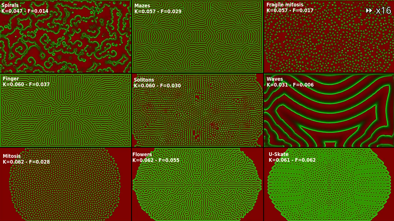
Some smart people have already studied the Gray-Scott model in-depth. And described the behaviors for some interesting parameter values. Most prominently :

• Robert Munafo hosts a methodic and exhaustive exploration of the Gray-Scott model’s parameter space. His website also features a gallery of videos for interesting parameter values.
• Karl Sims’ tutorial features some visual explanations.
• Katharina Käfer and Mirjam Schulz’s page features an interesting “Theory” section that includes some discussion about the model’s fixed points (conditions over which concentrations in both chemical species in a cell remain constant over time).

Their work has allowed me to quickly try out speed-constant values which produce interesting results. The video below showcases a few set of well-known parameters.

I strongly encourage you to check it out on Shadertoy. Experiment with different values for the speed constants k2 and k3 (in the “Common” tab) and see how adding some catalyst (green species) with your mouse changes the patterns.

Hacking on the code

Beyond simply tuning the values of k2 (\(K\)) and k3 (\(F\)), there are a few easy things to try (use the “Fork” button to save your changes to a new shader) :

• Change the initial conditions of the simulation and see how they influence the emerging behaviors for some given parameter values. The easiest way to do this is to change the source of iChannel2 in the “Buffer A” tab and change the channel2Init parameter in the “Common” tab
• Add new ways to interact with the simulation, such as :
  • A keyboard toggle for adding/removing the catalyst with the mouse
  • A key to switch between the catalyst (green) and the food (red) when using the mouse
  • A key to pause the simulation while maintaining the ability to interact with it
  • Different keys reset the simulation with a different initial state
• Control the scale of the simulation by expanding the diffusion neighborhood
• Use some generative noise to continuously add some perturbations to the simulation
• Try to reproduce the last piece of footage from the video (parameter space visualization). This only requires setting k2 and k3 to be proportional to the x and y coordinates. If you go one step further, you can even zoom into the most interesting regions of the parameter space.

Continuous cellular automata

You may have heard of Conway’s game of life in which a grid is repeatedly updated according to simple local rules in a binary way (the cells are either ON or OFF). This is an instance of a cellular automaton

Even though Conway’s game of life is much simpler than the reaction-diffusion model, complex patterns can still emerge from it such as the one in the animation above. Some people have even built logic gates in Conway’s game of life and used them to build Game of life inside Game of life

The Gray-Scott model can be seen as a continuous extension to the discrete version : instead of each cell’s state being represented with a value from a finite set of possible values, each cell’s state is now represented as two numbers from a continuum of possible values.

Other continuous cellular automata include the Lenia family and Flow Lenia which adds constraints enforcing some conservation of mass in the system. These kinds of models are actually used by scientific researchers to explore possible conditions for the emergence of proto-life.

Taking inspiration from the implementation I wrote for the Gray-Scott model, it should be possible to run a rudimentary version of other continuous cellular automata.

Conclusion

Although this can be considered an unorthodox use of shaders, this has been a great way to introduce myself to GPU programming. Being an implementation of concepts I’m already familiar with, I think this was much easier than dealing with the complex linear algebra involved in 3D rendering.

I hope to explore more systems that exhibit emergence in future posts, as I find this field really fascinating.